From Static Splats to Dynamic Worlds: The 4D Gaussian Frontier
How 4D Gaussian Splatting extends real-time radiance fields into the time domain — deformation fields, temporal regularization, neural scene flow, and the path to dynamic world models.
W16 Trend Tutorial | Difficulty: Advanced | Research area: Dynamic 3D reconstruction
Companion Notebooks
| Notebook | Title | Link |
|---|---|---|
| 00 | 4D Gaussians from Scratch: Adding Time to Gaussian Splatting | 00_4d_gaussians_from_scratch.ipynb |
| 01 | Video-to-3D: Reconstructing Dynamic Scenes from Synthetic Video | 01_video_to_3d_toy.ipynb |
1. Why Time Is the Next Frontier
Two weeks ago, W14 solved static 3D. Kerbl et al.'s 3D Gaussian Splatting (3DGS) achieved photorealistic reconstruction of static scenes at real-time framerates (100+ FPS). Last week, W15 showed us the architectures that power spatial reasoning: State Space Models, equivariant networks, and hybrids that move beyond pure attention.
But the real world moves. A person walks through a room. Cloth deforms. Reflections shift. A robot grasps an object and relocates it. Static reconstruction was the warm-up problem. Dynamic reconstruction is the prize.
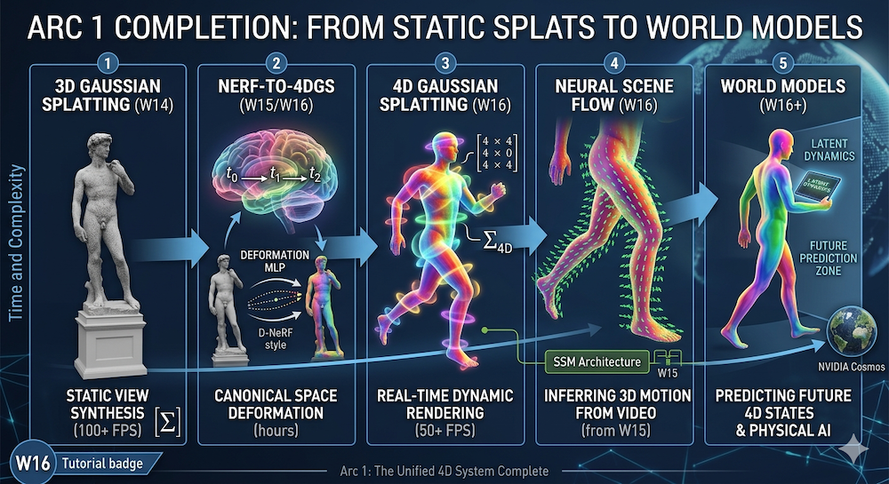
This week closes the first arc: W13 asked how AI should model the world (latent dynamics, world models) → W14 showed what to render (Gaussian splats) → W15 determined which architecture powers it (SSMs and beyond) → W16 addresses what every scene model must handle: time and motion.
The applications are immediate. Autonomous driving needs real-time 4D scene understanding from camera feeds. AR/VR requires dynamic environment reconstruction from video. Film VFX pipelines are replacing manual keyframing with learned deformations. Robotics simulators need physical-world models that predict how scenes evolve. Each demands one thing: a differentiable, real-time 4D (3D + time) representation learned from 2D video.
The core challenge: Given multi-view video of a dynamic scene, learn a compact 4D representation that enables photorealistic view synthesis and forward simulation.
2. Recap: 3D Gaussian Splatting in 30 Seconds
A Gaussian Splat is defined by:
- Position:
- Covariance: , factored as where is a rotation (parameterized by a unit quaternion) and is an anisotropic diagonal scale. This keeps positive semi-definite through optimization while letting each splat be a stretched ellipsoid — essential for representing thin surfaces efficiently.
- Opacity:
- Color: Spherical harmonic (SH) coefficients for view-dependent appearance
The original 3DGS paper (Kerbl et al., 2023) showed that a set of thousands of Gaussians, optimized via gradient descent against multi-view image loss, converge to photorealistic novel views in minutes.
Rendering is the key insight: Project each 3D Gaussian to 2D screen space, apply the 2D covariance, compute opacity-weighted colors via front-to-back alpha compositing. No ray marching. No volume rendering integrals. Pure differentiable rasterization, GPU-optimized, 100+ FPS on consumer hardware.
The missing piece: Every Gaussian is frozen in space. , , , and color coefficients never change. Static scenes perfect. Dynamic scenes impossible.
3. The NeRF-to-4DGS Pipeline: How We Got Here
Before 3DGS, the NeRF ecosystem already tackled dynamics.
D-NeRF (Pumarola et al., 2021) introduced canonical space deformation: maintain a canonical NeRF of the scene at a reference time, then learn an MLP that maps positions at arbitrary times back to canonical space. This MLP is the deformation field. Training works: photometric loss drives the deformation field to align multi-view observations. But rendering takes minutes per frame.
Nerfies (Park et al., 2021) applied the same idea to casual monocular video—deformation fields without multi-view constraints. HyperNeRF (Park et al., 2022) extended deformations to higher-dimensional ambient spaces to handle topology changes (hair, fabric, foam).
All three work. All three are slow. Training takes hours. Novel-view synthesis takes seconds per frame. The question arrived naturally: can we achieve 3DGS's speed boost for dynamic scenes?
The answer: yes, but with four distinct flavors, each with tradeoffs.
4. 4D Gaussian Splatting: Four Approaches
At a glance, before we dig in:
| Approach | Core Mechanism | Best For | Main Bottleneck |
|---|---|---|---|
| 4.1 Deformation MLP | Canonical Gaussians + learned that warps them per frame | Medium-length clips with smooth motion; memory-constrained settings | MLP overfits / smears over long horizons; struggles with large nonrigid deformation |
| 4.2 Explicit Per-Frame Tracking | Independent Gaussians per timestep, tied together by rigidity / isometry losses | Long-range tracking, scene editing, large nonrigid motion | Memory grows as ; regularization tuning is delicate |
| 4.3 4D Spacetime Gaussians | One 4D Gaussian per primitive; render-time slice at gives a 3D Gaussian | Elegant, unified formulation; very smooth motion | Numerical conditioning of 4D covariance is the real headache (not topology); a single slice assumes unimodal temporal support |
| 4.4 Sparse Control Points | A small skeleton of control trajectories drives many Gaussians via interpolation | Interactive editing, rigged / skeletal subjects | Assumes low-dimensional motion manifold; weak on fluids, foam, fine cloth |
The sections below walk each in order.
4.1 Deformation Fields: The Direct Translation
Yang et al. (2024) applied D-NeRF's canonical-space idea directly to Gaussians.
Each Gaussian lives in canonical space at a reference time . At rendering time , a learned deformation field computes:
The deformation field is a small MLP, , parameterized as a hash-grid + linear layers for speed. Covariance and opacity deform similarly:
Training optimizes: , , , and the canonical Gaussian parameters against multi-view video loss (photometric + depth regularization).
Advantages: Clean conceptually. Minimal memory overhead (store one canonical set + tiny MLP). Renders at 30+ FPS. Disadvantages: Deformation fields can overfit, especially over long time horizons or with large nonrigid motion.
4.2 Explicit Per-Timestamp Gaussians: Independent Tracking
Dynamic 3D Gaussians (Luiten et al., 2024) sidestep deformation fields entirely.
Maintain an independent set of Gaussians at each timestep . No canonical space. No deformation MLP. Each frame's Gaussians are optimized directly.
The trick is regularization. Without constraints, Gaussians drift arbitrarily across frames. Two losses prevent this:
- Local Rigidity Loss: Neighboring Gaussians in space should move similarly.
- Isometry Loss: Distances between Gaussian pairs should be preserved (encourages rigid motion).
These soft constraints are cheap to compute and preserve speed.
Advantages: No deformation bottleneck; handles large nonrigid deformations better. Long-range tracking of individual Gaussians enables scene editing and object removal. Disadvantages: Memory scales as . For 300 frames and 100K Gaussians, this is substantial. Regularization tuning is delicate.
4.3 4D Gaussian Splatting: Time as a First-Class Dimension
Wu et al. (2024) proposed the most elegant solution: treat time as a fourth spatial dimension.
Instead of Gaussians, use Gaussians with mean and a full 4D covariance
so that a primitive is
The key intuition: rendering at time is a slice, not a marginal. Geometrically, fixing cuts a 3D ellipsoidal cross-section out of the 4D covariance ellipsoid. Statistically, this is conditioning , not marginalizing over . That distinction matters: a marginal would average the primitive over its entire temporal lifespan and hand back the static 3D shadow, which is not what you want to rasterize.
Using the standard Gaussian conditioning identities, the sliced 3D Gaussian has
The time-mean shift gives the primitive a built-in linear trajectory (the slope is the cross-covariance rescaled by temporal variance); the covariance shrinkage is a Schur complement — it's what's left of the spatial ellipsoid after the temporal direction is pinned. This sliced 3D Gaussian then rasterizes normally through the 3DGS pipeline.
For both of those formulas to stay well-defined, has to remain positive semi-definite (PSD) throughout training. In practice this is enforced by factoring (the 4D analogue of the quaternion + scale factorization from §2), which is why the numerical-conditioning worry in the table is real — sloppy parameterizations can drift into near-singular 4D covariances and blow up at slice time.
Advantages: Mathematically elegant. Inherits 3DGS's real-time rendering (50+ FPS). Temporal continuity is built into the primitive itself, not added on top. Disadvantages: A single 4D Gaussian implicitly assumes a unimodal temporal support, so motion that is long, nonlinear, or reappearing (think: occlusion/disocclusion) typically needs multiple primitives to cover it. The 4D covariance must be parameterized carefully to preserve PSD under gradient updates.
4.4 Sparse Control: Editable Deformations
SC-GS (Huang et al., 2024) targets interactivity. Rather than optimize millions of Gaussians, optimize a sparse control skeleton:
- Place control points (where ) in the scene.
- Connect them via a spatial graph.
- For each Gaussian, compute deformation as a weighted interpolation of nearby control-point motions.
- Each control point's trajectory is a curve: parameterized by a few keyframes or a B-spline.
Training optimizes control point trajectories and the interpolation weights.
Advantages: Interactive editing (move a control point, scene deforms naturally). Explainable (users see what they're controlling). Renders in real time. Disadvantages: Assumes skeletal structure (works for people, furniture; breaks for fluids, cloth folds). Less photorealistic than end-to-end optimization.
5. Neural Scene Flow: Motion from Video
The deformation field in Section 4.1 computes scene flow: the per-point 3D motion in a scene, generalizing 2D optical flow to 3D.
RAFT (Teed & Deng, 2020) showed that iterative correlation-volume refinement powers optical flow estimation on 2D images. It became the backbone of modern flow networks.
Neural Scene Flow Fields (Li et al., 2021) extended this to 3D: learn a NeRF-like MLP that predicts per-ray 3D motion from monocular video. Given two frames, estimate depth at each pixel, then look up scene flow to predict the 3D motion.
Connection to 4D Gaussians: The deformation field is scene flow. Scene flow answers: "at position , how is the scene moving?" Gaussians encode the scene; scene flow encodes its dynamics.
Connection to W15 (architectures): Last week's SSMs and equivariant networks map almost directly onto the bottleneck we flagged in §4.1 — deformation MLPs that overfit or smear over long time horizons. A per-Gaussian MLP has no explicit notion of sequence; it treats as an arbitrary 4D input. A State-Space Model, by contrast, is a temporal primitive: it carries a compact hidden state forward, scales linearly in sequence length, and is designed to remember long contexts without a quadratic attention bill. Swap the deformation MLP for an SSM that ingests as a trajectory and you get a deformation field that can actually reason about minute-long clips instead of just a few seconds. Equivariant networks add the complementary piece: rotations and reflections of the scene leave the predicted motion equivariantly rotated and reflected, which is exactly the inductive bias you want for rigid + articulated content. SSMs handle the long axis; equivariant layers handle the spatial symmetries 4D Gaussians should respect anyway.
6. From 4D Reconstruction to World Models
4D Gaussians solve inverse problem: given video, infer the 4D structure. World models solve the forward problem: given current state, predict future states.
NVIDIA Cosmos is a diffusion-based world foundation model for physical AI. It predicts video frames conditioned on past frames and action inputs. Its strength: learned physics intuition. Its weakness: pixel-level generation is diffusion-slow.
V-JEPA 2, Meta's follow-up to JEPA, sidesteps pixels entirely. It operates on learned representations and predicts latent dynamics without committing to pixel space.
DreamZero (Ye, Ge et al., 2026) reframes the question as "what will happen if I take this action?" — a World Action Model built on a video-diffusion backbone that jointly predicts future frames and actions, and transfers zero-shot across new tasks and embodiments.
The convergence point: 4D Gaussians provide the rendering engine (fast, differentiable 4D-to-2D projection). World models provide the dynamics engine (predict future 4D states). Stack them:
- Observe video → reconstruct 4D Gaussians (inverse problem).
- Feed current Gaussian state to world model → predict next-timestep Gaussians (forward problem).
- Render predicted Gaussians to generate future video for loss computation.
This loop is the foundation for embodied AI. Physical Intelligence's π0 demonstrated this: a robot foundation model trained on diverse manipulation videos, learning implicit world models that enable zero-shot generalization.
The full circle: W13 asked how AI models dynamics → W14 showed how to render efficiently → W15 proved which architectures scale → W16 combines them into a unified 4D system.
7. What We Build This Week
Notebook 00: 4D Gaussians from Scratch
We extend W14's static Gaussians with a time dimension:
- Synthetic data generation: 50 canonical Gaussians following a mix of sinusoidal, linear, and circular trajectories — circular is the hard case because it forces the MLP to learn nonlinear time dependence.
- Deformation MLP: A tiny deformation field (2-layer ReLU MLP, 64 hidden units, ~4.5k parameters) in NumPy with explicit forward and hand-written backward passes — no autodiff.
- Training loop: Gradient accumulation across timesteps + cosine learning-rate decay, MSE loss against noisy 2D observations.
- Regularization: Velocity penalty and the jerk-vs-fidelity tradeoff it creates.
- Visualization: Static (3DGS-style) vs. dynamic (4DGS-style) reconstructions side-by-side — the dynamic model beats the static mean-position baseline by ~39% at every timestep.
By notebook's end, you'll have intuition for why deformation fields work and where they fail (e.g., occlusion boundaries, rapid topology changes).
Notebook 01: Video-to-3D Toy Pipeline
We build a minimal, pure-NumPy video-to-3D pipeline on a synthetic scene — the goal is to expose the mechanics of lifting 2D motion into 3D, not to benchmark against state of the art:
- Scene generation: Synthetic 20-frame sequence — a translating sphere, a rotating cube, and a fixed background — with a pinhole camera.
- Optical flow: Compute ground-truth 2D flow analytically, as the pixel difference between consecutive projections. (We reach for RAFT/MiDaS-style learned flow + depth in a later week; here we use the analytical ground truth to keep the rest of the pipeline readable.)
- Lifting flow to 3D: Invert the pinhole projection using the known depth to recover scene-flow and components per point; the component stays as a placeholder and motivates the depth-ambiguity callout.
- Temporal propagation: Forward-integrate per-frame flow to build a temporal point cloud; compare the lifted trajectory to the ground-truth scene flow.
- Drift diagnosis: Quantify error growth over 20 frames and explain why frame-by-frame integration drifts without a global optimization loop (the opening for 4DGS / NSFF).
- Static vs. flow-aware baseline: Compare a "repeat " baseline against flow-based propagation; at , flow-aware is ~29× better by MSE.
- Smoothing: Apply moving-average temporal smoothing (single- and two-pass) to damp noise, and use it to preview why learned temporal regularization beats hand-rolled filters.
This notebook closes the loop from W13 → W16 at toy scale: from "how do world models work?" to "what are the mechanical steps of reconstructing one from video, and where do they break?"
8. Conclusion: The Arc Completes
- W13: World models landscape — how should AI model dynamics? Latent vs. pixel space, world models as foundation models.
- W14: 3D Gaussian Splatting — what representation enables real-time photorealistic rendering? Splats, not voxels or meshes.
- W15: Post-Transformer Architectures — which architectures power spatial reasoning? SSMs, equivariance, hybrids that outpace attention.
- W16: 4D Gaussian Splatting — what about time? Deformation fields, scene flow, the marriage of inverse (reconstruction) and forward (prediction) problems.
Arc 1 is complete. We now have:
- A rendering primitive that is fast and differentiable (3DGS).
- A temporal extension that preserves that speed (4D-GS).
- Architectures that naturally model sequences (SSMs).
- The conceptual framework to connect reconstruction to prediction (world models).
Coming up in this series: The Probabilistic Renaissance — Gaussian processes, uncertainty quantification, and why the field is rediscovering Bayesian methods. See Attention Is All You Need… Is a Kernel and the W28 uncertainty trio.
Sources & Further Reading
Core 4D Gaussian Papers:
- 3D Gaussian Splatting for Real-Time Radiance Field Rendering (Kerbl et al., 2023)
- 4D Gaussian Splatting for Real-Time Dynamic Scene Rendering (Wu et al., 2024)
- Deformable 3D Gaussians for High-Fidelity Monocular Dynamic Scene Reconstruction (Yang et al., 2024)
- Dynamic 3D Gaussians: Tracking by Persistent Dynamic View Synthesis (Luiten et al., 2024)
- SC-GS: Sparse-Controlled Gaussian Splatting for Editable Dynamic Scenes (Huang et al., 2024)
Dynamic NeRF Foundations:
- D-NeRF: Neural Radiance Fields for Dynamic Scenes (Pumarola et al., 2021)
- Nerfies: Deformable Neural Radiance Fields (Park et al., 2021)
- HyperNeRF: A Higher-Dimensional Representation for Topologically Varying Neural Radiance Fields (Park et al., 2022)
Scene Flow & Optical Flow:
- RAFT: Recurrent All-Pairs Field Transforms for Optical Flow (Teed & Deng, 2020)
- Neural Scene Flow Fields for Space-Time View Synthesis of Dynamic Scenes (Li et al., 2021)
World Models & Prediction:
- NVIDIA Cosmos
- World Action Models are Zero-shot Policies — DreamZero (Ye, Ge et al., 2026)
- NeRF: Representing Scenes as Neural Radiance Fields for View Synthesis (Mildenhall et al., 2020)
Related Artifocial Tutorials:
- W13: World Models Landscape
- W14: Gaussian Splatting Explained
- W14: Image-to-3D Landscape
- W15: Beyond Attention – Post-Transformer Architectures
- W15: SSM vs. Attention Notebook
Stay connected:
- 📧 Subscribe to our newsletter for updates
- 📺 Watch our YouTube channel for AI news and tutorials
- 🐦 Follow us on Twitter for quick updates
- 🎥 Check us on Rumble for video content