4D Gaussian Splatting Explained: Extending 3DGS to the Time Domain

Level: Intermediate | Prerequisite: Gaussian Splatting Explained (W14)

Companion Notebook

Notebook	Topic
00_4d_gaussians_from_scratch.ipynb	Pure NumPy deformation-based 4DGS on synthetic data

1. From Photographs to Movies

In the W14 basics, we learned that 3D Gaussian Splatting (Kerbl et al., 2023) reconstructs a frozen moment from a set of photographs. You point a camera at a scene, capture multiple views, and 3DGS gives you a real-time, high-fidelity 3D representation you can render from any angle.

But the world is not frozen. People walk, objects fall, lighting changes. Leaves sway in the wind. Clothes deform as an actor moves. If you try to apply 3DGS to a video sequence frame-by-frame, you'll get flickering and artifacts because each frame's Gaussians are learned independently, with no awareness of motion continuity.

This is where 4D Gaussian Splatting comes in. By adding a temporal dimension, we learn Gaussians that change over time. Instead of "here's what the scene looks like at frame 42," we say "here's how the scene evolves from frame 1 to frame 100." The result: real-time rendering of dynamic scenes, often at 30–60+ FPS.

This article explains the core ideas and strategies. The companion notebook builds a working deformation-based 4DGS model from scratch, showing exactly how temporal deformation works.

2. Quick Recap: What Is a 3D Gaussian?

If you've read the W14 basics, you know the essential parts. A 3D Gaussian in space is defined by:

Position: $\mu = (x, y, z)$
Covariance: $\Sigma$ (shape and orientation), usually factored as rotation $q$ (quaternion) and anisotropic scale $s = (s_x, s_y, s_z)$ — per-axis scaling is what lets one Gaussian cover a thin wall or a long hair strand instead of packing many spheres to do the same job
Opacity: $\alpha \in [0, 1]$
Color: Spherical harmonic (SH) coefficients $c_0, c_1, \ldots$

Rendering works by:

Projecting each Gaussian to 2D screen space
Sorting by depth
Alpha-compositing in order

The entire pipeline is differentiable, so we can backprop photometric losses through the renderer and update the Gaussian parameters.

For a refresher on the math and why splatting is fast, see Gaussian Splatting Explained (W14).

3. Adding Time: The Core Idea

To extend 3DGS to dynamic scenes, the key insight is simple: make every Gaussian property a function of time $t$ .

Instead of fixed $\mu, \Sigma, \alpha, c$ , we now have:

$\mu(t), \quad \Sigma(t), \quad \alpha(t), \quad c(t)$

At each frame, we evaluate these functions at the frame's timestamp and render as usual.

But how do we learn these time-dependent functions? Two strategies have proven effective:

Deformation fields: Start with canonical Gaussians and learn a time-dependent offset.
4D Gaussians: Treat time as a 4th spatial dimension and condition on the render-time $t$ to slice out a 3D Gaussian.

Let's explore both.

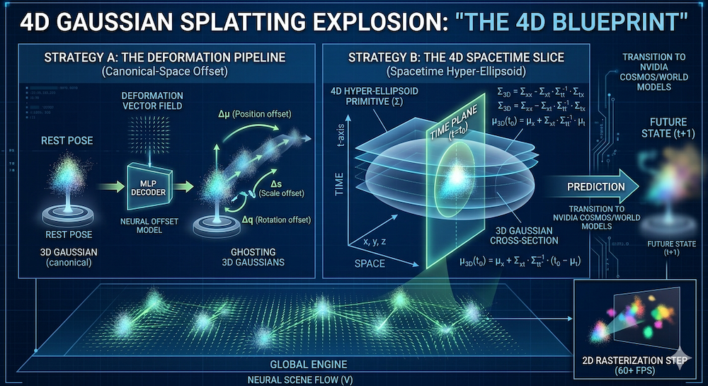
3.1 Strategy A: Deformation Fields

The deformation field approach is the most practical and widely adopted.

Idea: Keep a canonical set of Gaussians (think of them as a "rest pose"). Then, learn a function $D(\mu_{\text{canonical}}, t) \to (\Delta \mu, \Delta r, \Delta s)$ that predicts how each Gaussian deforms at time $t$ . In practice, most deformable-3DGS variants deform geometry only (position, rotation, scale) and keep appearance (opacity, color) static — this covers most motion (people walking, objects falling, cloth swaying) while keeping the deformation network small. Methods that also want time-varying lighting or color add a second, appearance-specific deformation head.

At time $t$ , the deformed Gaussian position is: $\mu(t) = \mu_{\text{canonical}} + \Delta\mu(t)$

Similarly for rotation and scale. The deformation function $D$ is typically a small MLP or other function approximator, applied per-Gaussian.

Training pipeline:

Initialize canonical Gaussians (e.g., from frame 0 or the scene's mean)
For each training frame at time $t$ $t$ :
- Evaluate $D(\mu_{\text{canonical}}, t)$ to get offsets
- Deform Gaussians using offsets
- Render the deformed Gaussians
- Compute photometric loss against the ground-truth frame
- Backprop through the renderer and the deformation function

This approach is described in Yang et al., 2024 (Deformable 3DGS). The deformation function can be as simple as a learned linear model or as complex as a neural network, depending on the scene's motion complexity.

3.2 Strategy B: 4D Gaussians

An alternative, more mathematically unified approach is to work directly in $(x, y, z, t)$ space.

Idea: Each Gaussian now has a 4D covariance matrix $\Sigma_{4 \times 4}$ . It describes the extent and orientation of the Gaussian not just in space, but also in time.

Geometric picture: slicing a 4D ellipsoid. Think of the level set of a 4D Gaussian as an ellipsoid in $(x, y, z, t)$ space. Rendering at a specific timestamp $t_0$ means cutting that 4D ellipsoid with the hyperplane $t = t_0$ — the cross-section is a 3D ellipsoid, which is exactly the 3D Gaussian you want to rasterize. Slice, not squash. Marginalizing out $t$ would flatten (integrate) the 4D ellipsoid into its static 3D shadow — effectively producing a "motion blur" that accounts for the Gaussian's existence across all time rather than its state at a specific instant. Conditioning on $t = t_0$ is the right operation, and it's cheap: a closed-form formula, no MLP call.

Mathematically, conditioning a 4D Gaussian on $t = t_0$ yields a 3D Gaussian with mean and covariance:

$\mu_{\text{3D}}(t_0) = \mu_x + \Sigma_{xt}\, \Sigma_{tt}^{-1}\, (t_0 - \mu_t)$

$\Sigma_{\text{3D}}(t_0) = \Sigma_{xx} - \Sigma_{xt}\, \Sigma_{tt}^{-1}\, \Sigma_{tx}$

where $\Sigma_{xx}$ is the spatial block of $\Sigma$ , $\Sigma_{tt}$ is the temporal variance, and $\Sigma_{xt}$ couples space and time. The mean drifts over time through $\Sigma_{xt}$ — that is how a 4D Gaussian encodes motion without an explicit deformation network. The covariance shrinkage (a Schur complement) is what's left of the spatial ellipsoid after the temporal direction has been pinned to $t_0$ .

The PSD catch. Both formulas above silently assume $\Sigma$ is positive semi-definite throughout training — otherwise $\Sigma_{tt}^{-1}$ isn't defined and the sliced covariance can blow up. Following the 3DGS convention, implementations parameterize $\Sigma = RSS^{T}R^{T}$ (the 4D analogue of the quaternion-rotation + anisotropic-scale factorization from §2), which guarantees PSD by construction under any gradient update. In the 4D analogue, $R$ is a $4 \times 4$ rotation matrix — unlike the 3D case where a single quaternion (4 parameters) suffices, 4D rotations have six degrees of freedom and are often handled via a pair of quaternions (left- and right-isoclinic rotations, sometimes called "4D rotors") or an explicit 6-parameter representation. This parameterization is what makes 4D Gaussians trainable in practice; drop it and numerical stability becomes the dominant failure mode.

This approach is presented in Wu et al., 2024 (4D Gaussian Splatting). The advantage is elegance and a unified representation; the disadvantage is that a single 4D primitive implicitly assumes unimodal temporal support, so motion that is long, nonlinear, or reappearing after occlusion typically needs multiple 4D Gaussians to cover — and the 4D covariance has to be parameterized carefully to stay PSD.

4. Training a 4DGS Model

Let's walk through a typical training loop (using deformation fields, the more common approach).

Input: Multi-view video (or monocular video with estimated camera poses)

For each training step:

Sample a frame at time $t$ and a camera viewpoint
Deform: Evaluate the deformation function for each Gaussian to get position $\mu(t)$ , rotation $r(t)$ , scale $s(t)$
Render: Use the standard splatting pipeline to render the deformed Gaussians to a 2D image
Photometric loss: Compare the rendered image with the ground-truth frame: $\mathcal{L}_{\text{photo}} = L_1(\hat{I}, I_{\text{gt}}) + \lambda_{\text{ssim}} (1 - \text{SSIM}(\hat{I}, I_{\text{gt}}))$ where $\hat{I}$ is the rendered image and $I_{\text{gt}}$ is the ground truth
Backpropagate: Gradients flow through the renderer, the deformation function, the Gaussian parameters, and the MLP weights
Update: SGD or Adam on all learnable parameters

The key difference from 3DGS is step 2 and the fact that the deformation function is now part of the computational graph.

Strategy A vs. Strategy B at a glance:

Feature	Strategy A (Deformation)	Strategy B (4D Spacetime)
Logic	Canonical splat + MLP offset	Spacetime ellipsoid slice at $t_0$
Per-frame cost	MLP eval + rasterize	Matrix ops + rasterize
Best for	Articulated motion (humans, hands)	Fluid / smooth motion (smoke, water)
Training stability	High — robust MLP optimization	Medium — needs PSD constraints on $\Sigma_{4\times4}$

In practice, many recent systems hybridize: a coarse 4D Gaussian provides the global trajectory and a lightweight deformation head corrects local detail.

5. Why Temporal Regularization Matters

Without constraints, the deformation function can do whatever it wants: it might make Gaussians teleport, spin wildly, or vanish between frames. This overfitting looks terrible.

Temporal regularization penalizes non-physical motion. Common regularizers include:

Velocity smoothness: Penalize the difference between deformations at adjacent frames: $\mathcal{L}_{\text{smooth}} = \sum_t \| D(\mu, t) - D(\mu, t-1) \|^2$ This encourages gradual, continuous motion.
Local rigidity: Nearby Gaussians should move similarly. This is based on the assumption that a rigid body part should deform coherently: $\mathcal{L}_{\text{rigid}} = \sum_{i,j \text{ nearby}} \| D(\mu_i, t) - D(\mu_j, t) \|^2$
As-rigid-as-possible (ARAP): A more sophisticated constraint: preserve local distances and angles between Gaussians. This is inspired by physics-based deformation and is particularly useful for cloth and skin.

Why does this matter? Think of it like a physics engine. Without temporal regularization, each frame is independent—like having no constraints on your simulation. With temporal regularization, you're adding springs and stiffness, ensuring that the motion is smooth and plausible. The regularization weight $\lambda$ is a tuning knob: higher $\lambda$ means stiffer, slower motion; lower $\lambda$ means more flexibility and faster adaptation to the data.

The total training loss is: $\mathcal{L}_{\text{total}} = \mathcal{L}_{\text{photo}} + \lambda_{\text{smooth}} \mathcal{L}_{\text{smooth}} + \lambda_{\text{rigid}} \mathcal{L}_{\text{rigid}}$

6. Rendering Dynamic Scenes in Real Time

One of the biggest wins of 4DGS over competing dynamic NeRF methods is speed.

Static 3DGS achieves 100+ FPS because splatting is embarrassingly parallel on the GPU. Each Gaussian is independent, so you can parallelize across thousands of Gaussians with ease.

4DGS adds exactly one step: evaluate the deformation function at time $t$ before rendering. Since the deformation MLP is tiny (typically 2–3 layers, a few hundred parameters), this is negligible:

$\text{Time} \approx \text{Deformation eval} + \text{Splatting} + \text{Compositing}$

The deformation eval is microseconds; splatting dominates, just like in 3DGS.

Result: 4DGS renders at 30–60+ FPS, depending on scene complexity. Compare this to the rough numbers reported in the original dynamic-NeRF papers:

Method	Approx. FPS	Approach
D-NeRF	~0.1	Full NeRF network + deformation MLP
Nerfies	~0.5	Deformation on learned NeRF features
4DGS	30–60+	Deformation on Gaussians + splatting

These are order-of-magnitude comparisons — exact numbers depend heavily on scene size, resolution, and hardware, so always consult the source papers for benchmarks in your setup. The order-of-magnitude takeaway holds: 4DGS makes dynamic scene rendering interactive for the first time.

2026 context: The ~100× speedup over D-NeRF has made 4DGS the de facto standard for real-time digital twin generation. Autonomous-driving pipelines, sports broadcast replay, and AR try-on systems that were previously NeRF-bottlenecked have largely migrated to Gaussian-based backends, and the gap continues to widen as custom CUDA splatting kernels mature.

7. Current Limitations and Open Problems

4DGS is powerful, but not a silver bullet.

Long sequences: Memory and computational cost scale with video length. High-quality reconstruction over minutes of footage is still challenging. Some approaches use hierarchical or streaming methods to mitigate this.
Topology changes: When objects appear or disappear (e.g., a door opening), a pure deformation field struggles because it assumes a fixed set of Gaussians. You'd need to explicitly handle creation/deletion of Gaussians, which is an active research area.
Monocular video: Without multiple views, depth is ambiguous. 4D reconstruction from a single camera is ill-posed unless you use strong priors (e.g., assume the scene is human-shaped). This is why most 4DGS methods target multi-view video or require camera poses.
Editing and control: How do you modify a single object (e.g., move the actor's arm) without affecting the rest of the scene? SC-GS (Huang et al., 2024) addresses this by segmenting Gaussians, but it's still an open problem.
Scale: City-scale dynamic scenes with multiple moving objects remain unsolved. Today's 4DGS works best on object-centric or room-scale scenes.

8. What We Build in Notebook 00

The companion notebook implements a deformation-based 4DGS from scratch, in NumPy, no frameworks.

Setup:

Synthetic data: 50 Gaussians following a mix of sinusoidal, linear, and circular trajectories (circular is the hard case — it requires the MLP to learn nonlinear time dependence)
2D orthographic projection — we intentionally drop perspective so the math stays focused on the temporal side; the notebook's engineering callouts explain when and why this simplification breaks down
Pure NumPy forward pass (no autodiff framework)
Explicit hand-written backprop — every shape and every ReLU derivative, no finite differences

You'll implement:

Initialization of canonical Gaussians
A 2-layer ReLU deformation MLP (64 hidden units, ~4.5k parameters)
Forward pass: deform → orthographic-project → compute MSE loss against noisy 2D observations
Training loop with gradient accumulation across timesteps and cosine learning-rate decay
Velocity regularization and its jerk-vs-fidelity tradeoff
Visualization: side-by-side comparison of static (3DGS-style) vs. time-aware (4DGS-style) rendering — the dynamic model beats the static baseline by ~39%

By the end, you'll see why motion matters: the static reconstruction flickers; the 4DGS reconstruction flows smoothly. And you'll have built it with no black boxes, just math and NumPy.

Summary

3DGS captures a frozen moment. 4DGS captures a movie. By making Gaussian properties functions of time, we unlock dynamic scene rendering.
Two main strategies: Deformation fields (practical, fast) and 4D Gaussians (elegant, sometimes less stable).
Temporal regularization is crucial. Without it, Gaussians overfit to individual frames. With it, motion is smooth and plausible.
Still real-time: Adding a deformation function adds microseconds. Splatting remains the bottleneck and remains fast. 30–60+ FPS is achievable even for complex dynamic scenes.
Open problems remain: Long sequences, topology changes, monocular reconstruction, and scene-scale editing are still active research areas.

The next step—moving from basics to trend analysis—will explore where dynamic scene understanding is heading: world models, multi-object tracking, and the path toward general video understanding.