Bayesian Rendering Explained: When a 3D Model Admits What It Doesn't Know
A beginner-friendly tour of Bayesian 3D reconstruction: why an ordinary 3D scan gives one confident answer everywhere, how turning geometry into a distribution produces honest confidence maps, and where the 'prior' that fills in unseen regions comes from.
Level: Beginner | Part of artifocial W29 Basics
The Map That Won't Admit It's Guessing
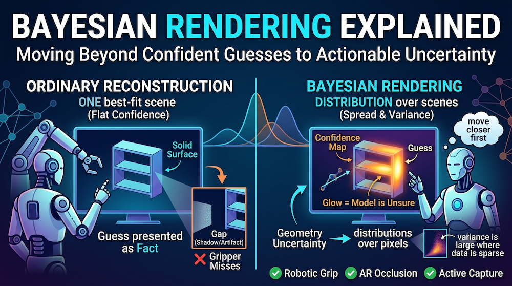
Picture a warehouse robot that has just built a 3D model of a shelf from a handful of camera snapshots. It needs to reach into a gap and grab a box. The model shows a clean, solid surface right where the robot wants to place its gripper — so it commits.
But the robot only ever photographed that gap once, from a steep angle, in shadow. The "solid surface" is a reconstruction artifact: a confident guess the model dressed up as a fact. The gripper closes on empty air, or worse, on something the model quietly smoothed away.
This is the central weakness of ordinary 3D reconstruction. It produces one model of the scene and presents every part of it with the same flat confidence — the corner you photographed from twenty angles and the corner you barely glimpsed look equally trustworthy. Last week we saw the same problem in 2D classifiers, which get more overconfident as they get bigger (Guo et al., 2017). This week it's geometry's turn. Bayesian rendering is how we teach a 3D model to say "I'm sure about this wall, but that gap? I'm guessing."
From One Scene to Many
Modern reconstruction methods like 3D Gaussian Splatting and NeRF work by tuning millions of numbers — positions, sizes, colors, opacities — until the model's rendered images match your photos as closely as possible. When the tuning finishes, you get a scene: the single configuration that best explains the pictures.
Here's the quiet assumption in that word "best." There are usually many scenes that explain your photos almost equally well, especially in regions you barely observed. Ordinary reconstruction reports just one of them — the single best-fit — and never quantifies how many others fit nearly as well. It's like a student who answers every exam question in the same confident handwriting, whether they studied the topic for a week or are pattern-matching a wild guess.
The Bayesian idea is to keep the alternatives. Instead of one number per parameter, we track a distribution — a best guess plus a spread that says how much wiggle room the data actually left. Where many cameras agree, the spread is tiny: the data pins the answer down. Where few cameras looked, the spread is wide: many scenes were consistent with what little you saw. That spread is the model's honesty, made quantitative.
Distributions Over Geometry Become Distributions Over Pixels
If every piece of geometry carries a spread, then so does everything you render from it. Point a virtual camera at a well-observed wall and every plausible version of the scene renders that wall the same way — the rendered pixels barely change. Point it at the under-observed gap and the plausible scenes disagree wildly — one fills the gap, another leaves it empty — so the rendered pixels swing all over the place.
That variation in the rendered image is a confidence map: a picture, in the same frame as your render, that glows exactly where the model is unsure. Distributions over geometry become distributions over pixels. You are no longer looking at a scene; you are looking at a scene and a map of where to trust it. For the warehouse robot, that map is the difference between "grab confidently" and "move closer and take another photo first."
Where Confidence Comes From: Agreement Between Views
How does the math decide a region is trustworthy without being told which parts you photographed well? The trick is to measure how much the answer resists change.
Take the finished model and imagine nudging one patch of geometry. If that nudge makes the rendered images clearly disagree with your photos, the data is holding that patch firmly in place — high confidence. If you can nudge it a lot and the rendered images barely flinch, the data never really constrained it — low confidence. Confidence is stiffness: how hard the observations push back when you try to move something.
Different methods measure that stiffness in different ways. Bayes' Rays perturbs a finished radiance field and watches how much the images resist, turning the result into a volumetric uncertainty field. FisherRF measures the same curvature to answer a second question ordinary reconstruction can't even ask: where should I photograph next? — namely, wherever the model is currently least sure. Both are computing the 3D version of the intuition from last week's Gaussian Processes: variance is large where data is sparse and small where it is dense.
Our companion notebook, Bayesian Gaussian Splatting, builds this end to end on a tiny toy you can run on a laptop: it fits a simple scene, deliberately leaves a region unobserved, and shows the confidence map lighting up over exactly that gap — while the model also, correctly, points at the gap when asked where to look next.
What To Do When You've Never Seen It: Priors
Confidence maps tell you where the model is guessing. They don't, by themselves, make the guesses any good. If no camera ever saw behind the couch, honest uncertainty says "wide spread here" — but a useful system still has to render something plausible, not a smear of noise.
That "something plausible" comes from a prior: a sense of what real scenes tend to look like, learned before any specific photo arrives. Couches have backs; walls are mostly flat; objects don't float. The modern way to capture that intuition is a diffusion or score model — the same family of models behind AI image generators. Trained on mountains of examples, it learns to nudge any configuration toward "looks like a real scene." Plug that prior into a Bayesian renderer and the unseen regions get filled with plausible structure instead of arbitrary filler.
When there's lots of data, the prior barely matters — the photos do the talking. When data is scarce, the prior does the heavy lifting, and it's the difference between a believable reconstruction and a hallucinated mess. Our second notebook, Score Matching Toy, builds a miniature score model from scratch and shows it learning to point toward where realistic data lives — the exact signal a sparse-view renderer leans on.
Why It's Worth the Trouble
Adding distributions to a 3D model costs real compute, and for a pretty fly-through demo it buys you nothing. It becomes essential the moment a decision rides on the geometry being real:
- A robot deciding where to grip needs to tell "definitely a surface" from "maybe an artifact."
- An AR headset placing a virtual object behind a real one must not trust a wall that isn't there.
- A scanning drone deciding where to fly next should head for the regions it's least sure about — active capture, guided by the confidence map.
In every case the useful question isn't "what is the geometry?" but "how sure are we, and where?" A reconstruction that can answer the second question is one you can actually act on. A splat that reports its own uncertainty is a small change to the pipeline — but it's the difference between a model that renders a confident guess and one that can say, honestly, I don't know what's back there yet.
This tutorial is part of the artifocial research-multimodal series. This week's advanced companion: When Gaussians Get Uncertain: Probabilistic 3D Reconstruction. Previous basics: Gaussian Processes Explained.
Build with AI — early access
Curious how uncertainty-aware models get built and shipped? Build with AI is our early-access program for engineers moving from tutorials like this to production AI — hands-on guidance instead of guesswork. Early access is opening now.